Digital Oscillator Deep Dive

Acton didn't attribute the formula to anyone, but Wikipedia calls it the "Chebychev method", citing Ken Ward's page on trigonmetric identities. He chose that name simply because Chebychev clearly knew the identity, but it was known well before him. Clay Turner calls it the "biquad oscillator" and attributes the formula to François Viète. Glen Van Brummelen also attribute this recurrence relation to Viète.

Boyer and Merzbach (2nd ed, p. 309) also attribute it to Viète and show his geometric proof of the Prosthaphaeresis Formulas from his Canon mathematicus published in 1579.³ These were used to quickly multiply (or divide) numbers by changing to an addition (or subtraction) and helped inspire logarithms for the same purpose. The formula using cosine is:

\[2\cos(A)\cos(B)=\cos(A+B)+\cos(A-B)\]

A simple rearrangement and setting \(A=n\theta\) and \(B=\theta\) gives the above form for the recurrence relation:

\[\cos(A+B)=2\cos(B)\cos(A)+\cos(A-B)\]

\[\cos((n+1)\theta)=2\cos(\theta)\cos(n\theta)-\cos((n-1)\theta)\]

However, Boyer and Merzbach attribute this cosine formula even earlier to the Egyptian mathematician ibn-Yunus around the year 1008 (2nd ed, p.240). His Wikipedia page also mentions this formula, but that is not currently reflected in the other Wikipedia pages.

Branko Ćurgus at WWU provides a neat and simple derivation of the recurrence relation using modern notation (see equation "(rr)").

Both Vicanek and Lyons provided a proof for the quadrature oscillator stability, but I have not seen a similar proof for the ibn-Yunus-Viète-Chebychev recurrence relation.

This is a block diagram for the Viète-Chebychev recurrence relation, with a dummy \(x(n)\) added⁴:

Here's a stability proof for the Viète-Chebychev recurrence relation that follows Lyons' proof fairly closely.

Starting with the trigonometric form of the recurrence relation:

\[\cos((n+1)\theta) = 2\cos(\theta)\cos(n\theta)-\cos((n-1)\theta)\]

Renumbering and renaming: \[y_n = 2\cos(\theta) y_{n-1} - y_{n-2}\]

Let \(k=2\cos(\theta)\).

\[y_n = k y_{n-1} - y_{n-2}\]

Finding the transfer function using Rick Lyons' fake \(x(n)\) impulse response trick:

\[y_n = k y_{n-1} - y_{n-2} + x_n\]

Take the z-transform:

\[Y(z) = k Y(z)z^{-1} - Y(z)z^{-2} + X(z)\]

Solve for \( H(z)=Y(z)/X(z) \): \[X(z) = Y(z) - k Y(z)z^{-1} + Y(z)z^{-2}\]

\[\frac{X(z)}{Y(z)} = 1 - k z^{-1} + z^{-2}\]

\[H(z) = \frac{Y(z)}{X(z)} = \frac{1}{1 - k z^{-1} + z^{-2}}\]

Multiply by \(z^2/z^2\) to get positive exponents: \[H(z) = \frac{z^2}{z^2 - k z + 1}\]

This gives two zeros at the origin and two poles.

Factoring to find the poles, we need to find \(a\) and \(b\) such that \(a b=1\) and \(a+b=-k=-2\cos(\theta)\):

\[H(z) = \frac{z^2}{(z+a)(z+b)}\]

Both \(k\) and \(1\) are real, so \(a+b\) is on the real axis. Because magnitudes multiply and phases add when multiplying complex numbers, \(|a|=|b|=1\), and \(\arg(a)=-\arg(b)\).

We can show that the complex conjugate pair \(1e^{\pm j \theta}\) satisfies these requirements using quadratic factorization (Lyons, p. 255):

\[f(s) = as^2 + bs + c = \\ \left( s + \frac{b}{2a} + \sqrt{\frac{b^2-4ac}{4a^2}} \right) \cdot \left( s + \frac{b}{2a} - \sqrt{\frac{b^2-4ac}{4a^2}} \right) \]

We have:

Since \(\cos^2(\theta) + \sin^2(\theta) = 1\), \(\sqrt{\cos^2(\theta)-1}=\sqrt{-\sin^2(\theta)}=j \sin(\theta)\).

So we have:

And so \(1 e^{\pm j\theta}\) are indeed the poles of our transfer function. Because the poles lie on the unit circle the system is stable.

The poles are never calculated directly, only \(2\cos(\theta)\) (and the initial outputs), so the poles will always land on the unit circle even with limitations in numerical precision. It's the structure of this recurrence relation that gives the stability. However, numerical precision will limit the frequency accuracy and lead to frequency drift from the desired frequency.

The disciminant of the quadratic formula determines whether the roots are complex or real. Because the range of cosine is \([-1, 1]\), the range of the discriminant \(b^2-4ac = 4\cos^2(\theta)-4\) is \([-4, 0]\). When the disciminant is negative, there are two complex conjugate roots. When the disciminant is zero, at the extreme of \(\theta=0\), those roots meet and form a single root at 1. In this case, the oscillator will output a constant value.

Beware of bugs in the above code; I have only proved it correct, not tried it.

–Donald Knuth

Of course I had to experimentally validate these oscillators and compare their performance.

For these experiments I have used a phase accumulator (unwrapped between 0 and \(2\pi\)) and sine and cosine functions as the reference signal. Of course, this will also drift somewhat from the ideal phase due to fixed numerical precision in the accumulator, but it is still a reasonable reference.

Note: The plots below use a sample rate of 44.1kHz, but I plan to replace them with normalized frequency plots in the future.

This plot shows how phase error (calculated with atan2()) accumulates in the Levine-Vicanek ("LV") and "Cheb" quadrature oscillators compared to the trig function phase accumulator at 1 kHz and a 44.1 kHz sample rate:

A few things to notice:

• The Cheb oscilator has a noisy sinousoidal component in their phase, likely from the two free-running sinusoids.
• The LV oscillator has a much less noisy phase error, because the two outputs are coupled and influence each other at each step. Vicanek mentions this effect in his paper.

The slope of the above graph varies with frequency, sometimes positive and sometimes negative. Sweeping over frequency and fitting a line to each slope gives the phase drift as a function of frequency for the two oscillators:

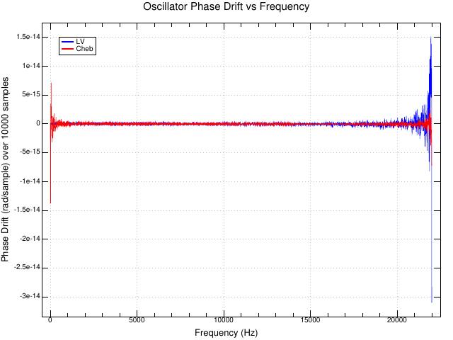
For the Levine-Vicanek oscillator, a 440 Hz tone at 44.1 kHz accumulates 1.68e-7 radians of error each second. At that rate it takes 11.6 years to accumulate a whole cycle of error.

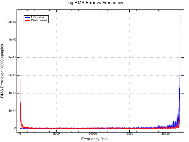
This plot shows the RMS error between the oscillator cosine outputs and the cos() trig function as a function of frequency:

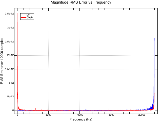
This plot shows the RMS error from the ideal complex manitude of unity for the two oscillators as a function of frequency:

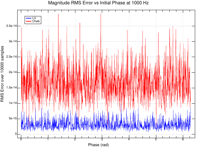
This plot shows the same RMS error from the ideal complex manitude of unity for the two oscillators, but as a function of starting phase at a fixed frequency of 1000 Hz:

For reference, this plot shows how poorly the trig functions perform when you neglect to unwrap the phase accumulator. It compares the output of the trig functions with and without unwrapping the phase accumulator. There are large jumps in phase error as the phase accumulator grows and the trig function produces less accurate results. Clearly the range reduction inside the library function isn't working well, and this makes sense when you consider that a large phase accumulator value has fewer bits of precision for the portion of the value modulo \(2\pi\).

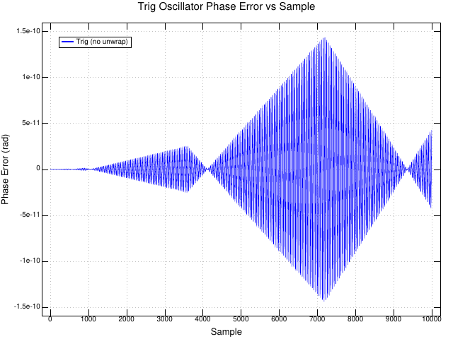
The takeaway here is that the drift performance of the two quadrature oscillators is quite good compared to sloppy handling of a phase accumulator and that phase accumulators should be unwrapped.

For these experiments I started with my usual blend of C, Awk, Make, and Gnuplot, but eventually switched to the J language, because it made exploring them faster. J is a descendent of APL, both designed by Ken Iverson and collaborators. I will post the C code in later post about my tides code.

The J code is in osc.ijs. This snippt shows the oscillator implementions:

NB. Levine-Vicanek Quadrature Oscillator
NB. Notation from "A New Contender in the Quadrature Oscillator Race"
NB. by Richard Lyons.

NB. f_hz:  oscillator frequency
NB. p_rad: phase
NB. s_hz:  sample rate
lv_init=: 3 : 0 "1
  'f_hz p_rad s_hz' =. y
  rps=.(2p1*f_hz)%s_hz                  NB. radians per sample
  rad=. 2p1#:!.0 p_rad                  NB. Unwrap phase.
  (2 o. rad), (1 o. rad), (3 o. rps%2), (1 o. rps)   NB. u v k1 k2
)

lv_step=: 3 : 0 "1
  'u v k1 k2'=. y
  w=.  u - k1 * v
  nv=. v + k2 * w
  nu=. w - k1 * nv
  nu, nv, k1, k2
)

lv_osc=: 3 : 0 "1
  0 lv_osc y
:
  NB. One-liner:
  NB. (j./)@:(2&{.)"1 lv_step^:(<x) lv_init y
  lv=. lv_step^:(<x) lv_init y
  (0{"1 lv) j. (1{"1 lv)
)


NB. Chebyshev Cosine Recurrence Relation
NB. From Acton, p. 173, Recurrence Relations.

NB. x:     1 for sine, 2 for cosine
NB. f_hz:  oscillator frequency
NB. p_rad: phase
NB. s_hz:  sample rate
NB. v0:    current value
NB. v1:    previous value
NB. k1:    step coefficient
cheb_init=: 3 : 0 "1
  2 cheb_init y
:
  'f_hz p_rad s_hz' =. y
  rps=.(2p1*f_hz)%s_hz                         NB. Radians per sample
  rad=. 2p1#:!.0 p_rad                         NB. Unwrap phase.
  (x o. rad), (x o. rad - rps), 2 * (2 o. rps) NB. v0 v1 k
)

cheb_step=: 3 : 0 "1
  'v0 v1 k'=. y
  ((k * v0) - v1), v0, k
)

cheb_osc=: 3 : 0 "1
  0 cheb_osc y
:
  cos=. {."1 cheb_step^:(<x) 2 cheb_init y
  sin=. {."1 cheb_step^:(<x) 1 cheb_init y
  cos j. sin
)

NB. Trig "oscillator"
NB. f_hz:  oscillator frequency
NB. p_rad: phase
NB. s_hz:  sample rate
NB. cos:   cosine
NB. sin:   sine
NB. rad:   phase in radians
NB. rps:   omega (radians per sample)
trig_init=: 3 : 0 "1
  'f_hz p_rad s_hz' =. y
  rps=.(2p1*f_hz)%s_hz                  NB. Radians per sample
  rad=. 2p1#:!.0 p_rad                  NB. Unwrap phase.
  (2 o. rad), (1 o. rad), rad, rps      NB. cos sin rad rps
)

trig_step=: 3 : 0 "1
  'cos sin rad rps'=. y
  rad=. 2p1#:!.0 rad+rps                NB. Increment and unwrap phase.
  (2 o. rad), (1 o. rad), rad, rps
)

trig_osc=: 3 : 0 "1
  0 trig_osc y
:
  trig=. trig_step^:(<x) trig_init y
  (0{"1 trig) j. (1{"1 trig)
)