A Fixed-Point Implementation of the Goertzel Algorithm in C
This is a practice project I did at the end of 2020. It's very on theme with the "Remcycles" moniker of this blog, because it's about a single tone detection algorithm, which detects "cycles" in a signal that occur at a specific frequency.
The Goertzel algorithm is a digital signal processing technique for calculating a single bin of a DFT/FFT. It's useful when you want to detect and measure the strength of a signal at just one or a few frequencies and don't need to calculate the signal strength at all the frequencies that an FFT would calculate. Possible use cases include decoding DTMF signals and demodulating on-off-keying or frequency shift keying signals.
I first read about it in this wonderful book by Richard Lyons:
Understanding Digital Signal Processing 3rd Edition
Lyons' book includes the following diagram, redrawn here using Pikchr and included via pikchr-mode (source code):

The structure above is a resonant filter. It's transfer function has a pole and zero that cancel each other, leaving a single pole on the unit circle: \[H(z) = \frac{(1 - e^{-j 2 \pi m/N}z^{-1})}{(1 - e^{+j 2 \pi m/N} z^{-1})(1 - e^{-j 2 \pi m/N} z^{-1})} = \frac{1}{1 - e^{+j 2 \pi m/N}}\]
That's a recipe for instability, but part of the Goertzel algorithm trick is to only run the filter for a fixed number of input samples before computing the final output, and then resetting the filter's state for the next set of samples.1
The following time-domain difference equations are the core of the algorithm and show how to calculate new values from previous values: \[w(n) = 2 cos(2 \pi m / N) w(n-1)-w(n-2) +x(n)\] \[y(n) = w(n) - e^{-j 2 \pi m / N} w(n-1)\]
The \(2 cos(2 \pi m / N)\) and \(e^{-j 2 \pi m / N}\) terms are constants that can be calculated once at run time (or even compile time), and \(y(n)\) only needs to be evaluated once at the end of each computation, after N+1 iterations of the main loop. Each iteration is only one multiplication and two additions.
I implemented this using floating-point math for practice first, but my goal was to write a fixed-point implementation that can run on microcontrollers or a DSP like the ADSP-BF706 without an FPU.
The two tricky parts of fixed-point programming are keeping the binary points aligned before and after operations and avoiding overflow. Randy Yates wrote two great guides on fixed-point math and signal processing that I highly recommend:
Fixed-Point Arithmetic: An Introduction
Practical Considerations in Fixed-Point FIR Implementations
There is also this helpful Wikipedia page on the different notations for fixed point numbers:
https://en.wikipedia.org/wiki/Q_(number_format)
My full test program used PortAudio for input and I used my system's audio mixer to route audio to it. The signal source was a simple direct digital synthesis (DDS) program that I wrote.
Here's a simplified version:
/* goertzel_fixed -- Detect a single tone in an audio signal.
   Copyright (C) 2022 Remington Furman
   This program is free software: you can redistribute it and/or modify
   it under the terms of the GNU General Public License as published by
   the Free Software Foundation, either version 3 of the License, or
   (at your option) any later version.
   This program is distributed in the hope that it will be useful,
   but WITHOUT ANY WARRANTY; without even the implied warranty of
   MERCHANTABILITY or FITNESS FOR A PARTICULAR PURPOSE.  See the
   GNU General Public License for more details.
   You should have received a copy of the GNU General Public License
   along with this program.  If not, see https://www.gnu.org/licenses/.
*/

#include <stdio.h>
#include <stdlib.h>
#include <stdint.h>
#include <math.h>
#include <complex.h>

/* These macros simplify working with signed fixed point numbers.

   In this notation, only the fractional bits are tracked in the macro
   names, so a Qm.n number is referred to as a Qn number, where n is
   the number of fractional bits.  This also sidesteps the issue of
   whether m includes the sign bit or not (ARM vs TI notation).

   The usual caveats of C preprocessor macros hold here.  Beware of
   multiple evaluations, side effects, etc.
*/

/* Convert to and from doubles. */
#define Qn_FROM_DOUBLE(value, n) (lrint((value) * (1 << (n))))
#define DOUBLE_FROM_Qn(value, n) ((double)(value) / (1 << (n)))

/* The number closest to +1.0 that can be represented. */
#define ONE_Qn(n) ((1<<(n)) - 1)
/* One half (0.5). */
#define HALF_Qn(n) (1<<((n) - 1))

/* Drop n bits from x (shift right) while rounding (add one half). */
#define ROUND_OFF_Qn(x, n)                      \
    ((n > 0) ? (((x) + HALF_Qn(n)) >> n) : (x))

/* Multiply two Qn numbers, rounding to the precision of the first.
   Make sure to cast one of the arguments to the size needed to avoid
   overflow in the multiplication before shifting. */
#define MUL_Qn_Qn(x, y, xn, yn)                 \
    ROUND_OFF_Qn((x) * (y), (yn))

/* Add two Qn numbers, using the precision of the first. */
#define ADD_Qn_Qn(x, y, xn, yn)                 \
    ((xn) > (yn) ? (x) + ((y) << ((xn)-(yn))) : \
     (x) + ROUND_OFF_Qn((y), ((xn)-(yn))))

typedef struct {
    int16_t real;
    int16_t imag;
} cint16_t;

/* Return a larger type here, because a complex point outside of the
   unit circle will have a larger magnitude. */
int32_t cint16_abs(cint16_t z) {
    /* Cheat for now and use floating point sqrt(). */
    return lrint(sqrt((double)z.real*(double)z.real +
                      (double)z.imag*(double)z.imag));
}

int16_t read_sample(void) {
    /* This function should read and return an audio sample from some
       source. */
    return 0;
}

int32_t goertzel(double detect_hz, double sample_rate_hz, int N) {
    /* Notation from p. 710 of Lyons. */

    /* Index of DFT frequency bin to calculate. */
    const double m = (N * detect_hz) / sample_rate_hz;

    /* This complex feedforward coefficient allows a single zero to
       cancel one of the complex poles.  It can be calculated in
       advance. */
    const double complex dbl_coeff_ff = -cexp(-I*2*M_PI*m/N);

    const int coeff_ff_Qn = 15;  /* Q1.15 */
    cint16_t coeff_ff;
    coeff_ff.real = Qn_FROM_DOUBLE(creal(dbl_coeff_ff), coeff_ff_Qn);
    coeff_ff.imag = Qn_FROM_DOUBLE(cimag(dbl_coeff_ff), coeff_ff_Qn);

    /* Feedback coefficient. */
    double dbl_coeff_fb = 2*cos(2*M_PI*m/N);
    const int coeff_fb_Qn = 14;  /* Q2.14 */
    int16_t coeff_fb = Qn_FROM_DOUBLE(dbl_coeff_fb, coeff_fb_Qn);

    const int w_Qn = 15;
    int32_t w[3] = {0};         /* Delay line. Q17.15. */

    int sample_index = 0;

    /* Read and process N+1 samples. */
    while (1) {
        const int x_Qn = 15;  /* Q1.15. */
        int16_t x = read_sample();

        if (sample_index == N) {
            /* The final x input sample should be forced to zero. */
            x = 0;
        }

        /* Manually shift delay line and calculate next value. */
        w[2] = w[1];
        w[1] = w[0];

        /* w[0] = x + (coeff_fb * w[1]) - w[2] */
        w[0] = MUL_Qn_Qn((int64_t)w[1], (int64_t)coeff_fb, w_Qn, coeff_fb_Qn);
        w[0] = ADD_Qn_Qn(w[0], x, w_Qn, x_Qn);
        w[0] = ADD_Qn_Qn(w[0], -w[2], w_Qn, w_Qn);

        if (sample_index++ == N) {
            /* End of Goertzel alogorithm for this buffer. Apply the
             * feedforward coefficient to generate final output. */
            const int y_Qn = 5;
            cint16_t y; /* y = w[0] + coeff_ff * w[1];  complex multiply. */
            y.real = ROUND_OFF_Qn(w[0] +
                                  MUL_Qn_Qn((int64_t)coeff_ff.real, w[1],
                                            coeff_ff_Qn, w_Qn), w_Qn - y_Qn);
            y.imag = ROUND_OFF_Qn(
                MUL_Qn_Qn((int64_t)coeff_ff.imag, w[1],
                          coeff_ff_Qn, w_Qn), w_Qn - y_Qn);

            int32_t dft_mag = cint16_abs(y);

            return dft_mag;
        }
    }
}

int main(void) {
    /* Input sample rate. */
    const double sample_rate_hz = 48000.0;

    /* Frequency of DFT bin to calculate. */
    const double detect_hz = 440.0;

    /* Number of samples for detection.  Need not be a power of 2. */
    const int N = 1024;

    while(1) {
        int32_t dft_mag = goertzel(detect_hz, sample_rate_hz, N);

        /* Normalize the DFT bin value by N.  A maximum amplitude
           signal at the detection frequency should give a value
           of 1/2. */
        double dft_mag_norm = dft_mag/N;
        printf("dft_mag: %u, dft_mag_norm: %g\n", dft_mag, dft_mag_norm);
    }
}
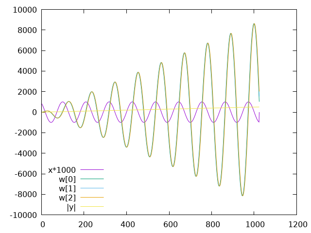
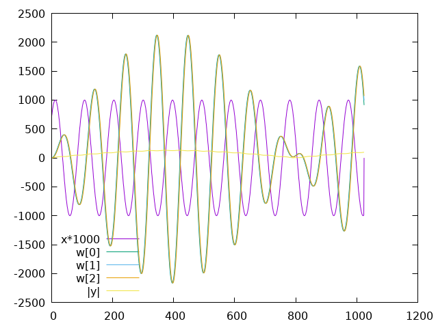
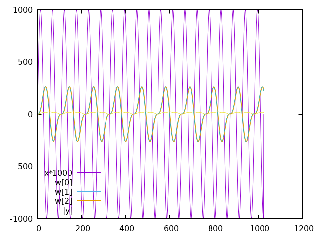
The following plots show the internal signals during each sample, with the final filter state on the right of each plot.
The yellow \(|y|\) trace is the output, the magnitude of the DFT bin, though it's poorly scaled to see relative to the other signals. The purple \(x\) trace shows the input signal scaled up to be more visible. The other traces are the internal filter state \(w\) values.
The filter is configured to detect a 440Hz tone, and the input signals are 440Hz, 500Hz, and 880Hz.

Figure 1: Goertzel state with 440Hz input
At 440Hz the input frequency matches the detection frequency and you can see that the internal filter state grows very quickly. It would continue to grow if the filter was run forever. The \(|y|\) trace steadily increases (again, hard to see with this scale).

Figure 2: Goertzel state with 500Hz input
At 500Hz input the filter state's magnitude oscillates, but never grows to a large value.

Figure 3: Goertzel state with 880Hz input
At 880Hz it also oscillates, but at a much smaller magnitude.
Footnotes:
There are still numerical instability problems with the basic algorithm (and refinements for avoiding them). See: https://academic.oup.com/comjnl/article-pdf/12/2/160/1021722/120160.pdf