The Geometry of the Smith Chart

I'm an embedded systems engineer and amateur radio operator and when I'm lucky I get paid to do electrical engineering work. One of the most interesting graph formats I've used is the Smith Chart. It has many uses for electrical engineering, including understanding antenna impedance measurements from a Vector Network Analyzer (VNA) and designing matching networks for mismatched antennas.

There are many resources on learning how to apply a Smith chart to RF engineering, and I won't attempt to write my own here. However, I found that most resources don't do a great job of explaining why the Smith chart is circular.

Most sources cite the familiar equation that relates the reflection coefficient \(\Gamma\) to a complex impedance \(z\):

\[\Gamma = \frac{z-1}{z+1}\]

But looking at that equation on it's own doesn't impart much intuition for why that leads to a circular chart.

Breaking the equation down, \(z-1\) shifts a complex point one unit to the left, and \(z+1\) shifts that point one unit to the right. Division of complex numbers is best done in polar coordinates, dividing the magnitudes and subtracting the phase angles (\(\frac{z_1}{z_2} = \frac{abs(z_1)}{abs(z_2)}e^{i(arg(z_1)-arg(z_2))}\)). But this still doesn't give much intuition as to what would happen to an entire half-plane of points when mapped with this equation.

The first document I found that make this click for me was this slide deck by Stephen D. Stearns, K6OIK:

Mysteries of the Smith Chart: Transmission Lines, Impedance Matching, and Little Known Facts

In particular, slides 29 and 30 make it graphically clear that the equation for \(\Gamma\) (and therefore, the Smith chart) maps the right hand side of the complex plane (that is, all points with non-negative real parts) to a unit circle. As it does this, it also shifts the point at (0,0) to (-1,0), so that the center of the circle is at (0,0). Points outside of this circle correspond to the left half of the complex plane, which aren't of interest for passive RF circuits, so they aren't shown on a Smith chart.

But the neat thing that really clicked for me was understanding that the vertical imaginary axis of the complex plane gets wrapped around the circumference of the Smith chart circle, with (0,0) moving the left hand side, (0,1) moving to the top of the circle, (0,-1) to the bottom, and the two points at infinity on the ends of the imaginary axis meeting at the right side of the circle.

From that epiphany, what I wanted to see next was an animation of this mapping taking place. I couldn't find one online, and I set that particular problem aside for a while. But recently I figured out a way to slowly apply the mapping so that I can watch the transformation take place and I wrote the code to do so.

This is the result:

The mapping is known as a Mobius transformation, and the general case of a Mobius transformation is:

\[\frac{a z + b}{c z + d}\]

And the general case of the Smith chart the equation is:

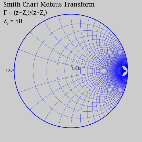
\[\Gamma = \frac{z-Z_0}{z+Z_0}\]

Thus, we have a Mobius transformation with \(a=c=1\) and \(d=-b=Z_0\).

Usually, \(z\) is normalized by dividing by the characteristic impedance of a transmission line (\(Z_0\)) before applying the transformation, and so the equation from the beginning of the article is the most frequently published.

But I noticed that if \(Z_0\) is very large, then for smaller values of \(z\) the transformation does not move the point very much (except for the leftward shift by 1). Drawing a connected Cartesian grid and mapping the grid points with smaller and smaller values of \(Z_0\) results in an animation like this:

Here, the grid is drawn with a line every ten units from \(0 \leqslant x \leqslant 1000\) and \(-1000 \leqslant y \leqslant 1000\), and the resulting circle is always scaled to fit in the frame of image. Because of the scaling, the grid appears to change size which is unfortunate, but it clearly shows how the points along the vertical imaginary axis begin to envelop the circle as the transform gets closer and closer to the target \(Z_0\). With large values of \(Z_0\), the grid is more or less rectangular (occupying only a small arc of the circle).

This grid chart is a little unsatisfying, since the grid points start to look angular as they get more separated. Plus, the constant diameter of the plot hides the fact that the points at infinity come closer and closer to the mapped (0,0) origin of the plot.

In order to keep the circular nature of the mapped grid lines I needed to work out the geometry (centers, radii, and angles) of the arcs after the mapping. This was a fun math problem, especially the arc lengths for proper clipping.

The vertical lines of the Cartesian grid map to circles with centers on the real axis to the right of (0,0), and they all pass through (1,0). The left most point of the circle passes through \(\Gamma = \frac{(x+0i)-1}{(x+0i)+1}\). From there, it's easy to calculate the radius and center of the circle.

The horizontal lines are a bit more complicated. The centers are all above (1,0), and they all pass through (1,0) as well. The other point they pass through is \(\Gamma = \frac{(0+y i)-1}{(0+y i)+1}\). A little of bit of algebra (Pythagorean Theorem) shows that the radius of the circle is \(r = \frac{(\Re(\Gamma)-1)^2 + \Im(\Gamma)^2}{2 \Im(\Gamma)}\). Finding the arc angle for clipping just involves the arctangent, since we know the two points that the arc must connect.

# Draw a series of Mobius transformations of a regular Cartesian grid
# to illustrate how a Smith chart is formed and how it relates to
# Cartesian space.
#
# Copyright Remington Furman, 2019-11-27.

using Cairo

plot_width  = 500
plot_height = 500
plot_scale  = 200

c = CairoRGBSurface(plot_width, plot_height);
cr = CairoContext(c);

gamma(z,n) = (z-n)/(z+n)

function connect_dots(dots)
    move_to(cr, real(dots[1]), imag(dots[1]))
    for dot in dots[2:end]
        line_to(cr, real(dot), imag(dot))
    end
    stroke(cr)
end

function connect_grid(grid)
    foreach(connect_dots, eachrow(grid))
    foreach(connect_dots, eachcol(grid))
end

function plot_smith_chart(n)
    set_source_rgb(cr,0.8,0.8,0.8) # Light gray background.
    rectangle(cr,0.0,0.0,plot_width,plot_height)
    fill(cr)

    set_line_width(cr, 0.5)     # Plot with thin blue lines.
    set_source_rgb(cr, 0,0,1)

    # Setup graphics transform matrix.
    save(cr)
    translate(cr, plot_width/2-plot_scale, plot_width/2) # Center the plot.
    scale(cr, plot_scale, plot_scale)                    # Embiggen.
    translate(cr, 1.0, 0.0) # A Smith chart maps 0+0j to -1+0j.  Undo that.

    # Make a regular grid.
    step = 10
    grid = [x+y*im for y=-1000:step:1000, x=0:step:1000]

    # Map the grid points and connect the dots.
    connect_grid(map(z -> gamma(z, n), grid))
    restore(cr)

    # Label plot.
    set_source_rgb(cr, 0,0,0)
    set_font_face(cr, "Noto Serif 16")
    line_space = 30
    text(cr, 12, 1*line_space, "Smith Chart Mobius Transform")
    text(cr, 12, 2*line_space, set_latex(cr, "\\Gamma  = (z-Z_0)/(z+Z_0)", 12), markup=true)
    text(cr, 12, 3*line_space, set_latex(cr, "Z_0 = $n", 12), markup=true)

    # Write it out to a file.
    write_to_png(c,"smith_grid_$n.png")
end

foreach(plot_smith_chart, [50, 100, 200, 500, 1000, 2000, 5000, 10000])

# Draw a series of Mobius transformations of a regular Cartesian grid
# to illustrate how a Smith chart is formed and how it relates to
# Cartesian space.
#
# Copyright Remington Furman, 2019-11-29.

using Graphics, Cairo

plot_width  = 500
plot_height = 500
plot_scale  = 4
clip = true

c = CairoRGBSurface(plot_width, plot_height);
cr = CairoContext(c);

gamma(z,n) = (z-n)/(z+n)

circle(ctx::CairoContext, xc::Real, yc::Real, radius::Real) =
    arc(ctx, xc, yc, radius, 0, 2*pi)

function map_vertical_line(x, n)
    set_line_width(cr, x==0 ? 2 : 0.5)
    max_diam = 2*n
    g = gamma(x+0*im,n)

    xg = n*real(g)
    yg = n*imag(g)

    r = (max_diam - (xg+n))/2
    xc = max_diam - r
    yc = 0
    circle(cr, xc, yc, r);
    stroke(cr)
end

function map_horizontal_line(y, n)
    set_line_width(cr, y==0 ? 2 : 0.5)
    if (y==0)                   # Special case: x-axis
        if (clip)
            move_to(cr, 0, 0)
            line_to(cr, 2*n, 0)
        else
            move_to(cr, -plot_width, 0)
            line_to(cr,  plot_width, 0)
        end

        stroke(cr)
        return
    end

    g = gamma(0+y*im,n)
    xg = n*real(g)
    yg = n*imag(g)


    yc = ((xg-n)^2 + yg^2)/(2*yg)
    xc = 2*n
    r = abs(yc)

    arc_deg = abs(2*atan(-yg, n-xg))

    if (clip)
        if (yc>0)
            end_deg = deg2rad(270)
            arc(cr, xc, yc, r, end_deg-arc_deg, end_deg);
        else
            end_deg = deg2rad(90)
            arc_negative(cr, xc, yc, r, end_deg+arc_deg, end_deg);
        end
    else
        circle(cr, xc, yc, r);
    end

    stroke(cr)
end

function text_vc_hr(cr, x, y, str)
    extents = text_extents(cr, str)
    xt = x - (extents[3] + extents[1])
    yt = y + extents[4]/2
    text(cr, xt, yt, str)
    move_to(cr, 0, 0)           # End the path.
end

function text_vb_hc(cr, x, y, str)
    extents = text_extents(cr, str)
    @show str, extents
    xt = x + (extents[3]/2 - extents[1])/4
    yt = y
    text(cr, xt, yt, str)
    move_to(cr, 0, 0)           # End the path.
end

function plot_smith_chart(n)
    set_source_rgb(cr,0.8,0.8,0.8) # Light gray background.
    rectangle(cr,0.0,0.0,plot_width,plot_height)
    fill(cr)


    # Setup graphics transform matrix, and label points of interest.
    save(cr)
    translate(cr, (plot_width-400) / 2, plot_width/2) # Center the plot.
    set_font_face(cr, "Noto Serif 10")
    set_source_rgb(cr, 0.2,0.2,0.2)
    text_vc_hr(cr, 0, 0, "(0,0)")                     # Label (0,0).
    scale(cr, plot_scale, plot_scale)                 # Embiggen.
    text(cr, n*(1+real(gamma(50,n))), 0, " (50,0)")   # Label (50,0).
    move_to(cr, 0, 0)

    # Map and plot the grid lines.
    set_source_rgb(cr, 0,0,1)
    step = 10
    foreach(x -> map_vertical_line(x,n), 0:step:50*step)
    foreach(y -> map_horizontal_line(y,n), -50*step:step:50*step)
    restore(cr)

    # Label plot.
    set_source_rgb(cr, 0,0,0)
    set_font_face(cr, "Noto Serif 16")
    line_space = 30
    text(cr, 12, 1*line_space, "Smith Chart Mobius Transform")
    text(cr, 12, 2*line_space, set_latex(cr, "\\Gamma  = (z-Z_0)/(z+Z_0)", 12), markup=true)
    text(cr, 12, 3*line_space, set_latex(cr, "Z_0 = $n", 12), markup=true)

    # Write it out to a file.
    write_to_png(c,"smith_circle_$n.png")
end

foreach(plot_smith_chart, 50:1:55)
foreach(plot_smith_chart, 55:5:80)
foreach(plot_smith_chart, 80:10:100)
foreach(plot_smith_chart, 200)
foreach(plot_smith_chart, 300:200:1000)
foreach(plot_smith_chart, 1000:1000:5000)