An Analog Computer Circuit for the SIR Model
Introduction
This is my obligatory coronavirus post.
After reading the Wikipedia page about the SIR model used as a simple epidemiology model for the spread of disease, I realized I might be able to make an analog computer circuit to simulate the model using a few op-amp integrators and a multiplier IC. I got this idea because I had previously built Paul Horowitz's fun Lorenz attractor circuit which does the same thing but for different equations.
For this project, I was mostly interested in determining the circuit topology necessary for simulating the model and getting qualitative results from the output, not quantitative results or usefully scaled numbers. The simulated circuit produces graphs very similar to a lot of the graphs produced by numerical software, and I am happy with the result.
This project required me to re-learn and practice some of my calculus from college, especially integration, which occurs less often in the problems I usually solve. Not only that, but I also started to actually understand some of the concepts for the first time or more deeply than I did before, even though I could previously go through the motions and complete the homework and tests in college1.
The SIR model
As mentioned, the SIR model uses differential equations to model the spread of disease. For a population of N people, there are three subpopulations: \(S\) for those susceptible to the disease (no immunity), \(I\) for those currently infected, and \(R\) for those who have recovered from the disease and developed immunity, or more unfortunately died and can no longer be infected again for that reason.
Let's look at the equations:
\begin{align*} \frac{dS}{dt} &= \frac{-\beta}{N} I S \\ \frac{dI}{dt} &= \frac{\beta}{N} I S - \gamma I \\ \frac{dR}{dt} &= \gamma I \end{align*}These equations define the rate of change for the three populations based on the size of the other two populations.
A great introduction to the SIR model is this video by Steven Brunton: https://www.youtube.com/watch?v=jmfsSmHAQ2o&t=372s
Integral form
The trick is realizing that we can integrate (or take the antiderivative of) both sides of each equation to give something we have a chance of implementing with op-amp circuits. Through the fundamental theorem of calculus, the integral of \(\frac{dS}{dt}\) is simply \(S(t)\) 2, and the integrals of two equal things are also equal.
\begin{align*} S &= \int \frac{-\beta}{N} I S dt \\ I &= \int \frac{\beta}{N} I S - \gamma I dt = \int \frac{\beta}{N} I S dt - \int \gamma I dt \\ R &= \int \gamma I dt \end{align*}Notice that \(I\) is essentially defined in terms of the other two functions, and is one term negated and then subtracted by the other. This can be accomplished with the inverting amp and difference amp configurations for an op-amp.
Therefore, there are only two quantities we need to integrate here:
\begin{align*} &\int \frac{\beta}{N} I S dt \\ &\int \gamma I dt \end{align*}Pulling the constant factors out gives:
\begin{align*} \frac{\beta}{N} &\int I S dt \\ \gamma &\int I dt \end{align*}These integrals can be implemented with an integrator op-amp configuration if there are node voltages that represent \(I\) and \(R\).
Finally, there is one multiplication to perform for the term \(I S\). This can be done with a multiplication IC (like the AD633) that operates on those node voltages.
The \(I S\) term represents a pairing of all the infected people with all the susceptible people, and \(\frac{\beta}{N}\) represents the fraction of people who become infected from those pairings. That fraction is a function of physical distance between the pair and how infectious the disease is.
Initial conditions
One thing to remember about the antiderivatives of a function is that there are infinitely many of them. Recall that the an antiderivative of any function is one whose derivative is the original function, and that the derivative of a constant \(C\) is zero (it disappears).
For example, if \(f(x) = x + C\), then \(\frac{f(x)}{dx} = 1\), and the information provided by the constant \(C\) is lost. Only the slope of the function contributes to the derivative and any vertical offset is ignored. In a sense, some information is lost, though in this case it was never provided by the differential equations to begin with.
Looking at the equations again, there should be "constants of integration" included 3:
\begin{align*} S &= \int \frac{-\beta}{N} I S dt + C \\ I &= \int \frac{\beta}{N} I S - \gamma I dt + C \\ R &= \int \gamma I dt + C \end{align*}But what value should these constants have? It took me a little while to even ask myself this question, but after a little thought it was clear.
The Wikipedia page points out the obvious, which is that the sum of all the sub-populations is the size of the total population.
\[ S + I + R = N \]
So, adding up all the equations should result in the number \(N\).
Another thing to notice is that the equation for \(S\) without the constant \(C\) would be negative, but a negative population size does not make sense. If the integration constant for \(S\) were \(N\), then \(S\) would always be positive, and \(S\) would represent starting with an entirely susceptible population, shrinking over time as people become infected and recovered. If the other integration constants are zero, then the sum of the three terms is indeed \(N\). In other words, in the beginning, everyone is susceptible (\(S=N\)), only one person is infected (\(I \approx 0\)), and no one is recovered (\(R=0\)).
Therefore, the equations to compute are4:
\begin{align*} S &= N - \int \frac{\beta}{N} I S dt \\ I &= \int \frac{\beta}{N} I S - \gamma I dt \\ R &= \int \gamma I dt \end{align*}Circuit components
Integrators
One of the basic building blocks provided by op-amps is an integrator:

Figure 1: Integrator
Looking again at Wikipedia, the voltage output of an op-amp integrator is:
\[ V_o(t) = V_o(0) - \frac{1}{R C} \int_0^t V_i dt \]
It's clear that the integrator inverts the input signal, but also scales it by a factor less than one. That scaling is very handy for our application because the constants \(\frac{\beta}{N}\) and \(\gamma\) are both less than one, and we can set the RC constants to equal the scaling constants from the equation. In other words:
\[ \frac{1}{R_1 C_1} = \frac{\beta}{N} \] \[ \frac{1}{R_2 C_2} = \gamma \]
And since a resistance is part of the RC constant, a potentiometer can be used to quickly change the constants in an actual circuit.
Inverting amps (multiplying by -1)
Because the integrators invert their input signals, we need to be invert them back to their positive values. Luckily, the inverting amplifier is another basic op-amp building block:

Figure 2: Inverting amplifier
If the two resistors are equal, then the output voltage is:
\[ V_o = - V_i \]
Difference amps (subtracting two values)
To subtract the \((N-S)\) and \(R\) signals and determine \(I\) we'll need yet another basic op-amp configuration, the difference amp:

Figure 3: Difference amplifier
If all four resistors have the same value, then the output voltage is simply:
\[ V_o = V_2 - V_1 \]
Simulated circuit and output
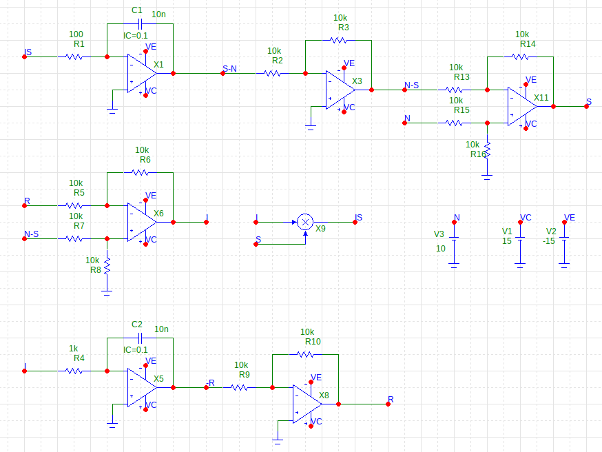
I used the wonderful (and now free, thanks to the generosity of Spectrum Software) Micro-Cap 12 circuit simulator to evaluate this circuit. For this simulation, I'm using a Spice macro that implements a perfect multiplier, rather than an AD633 IC. The op-amps are TL081C models.
Here is the schematic of the full SIR model circuit (click for full-res):
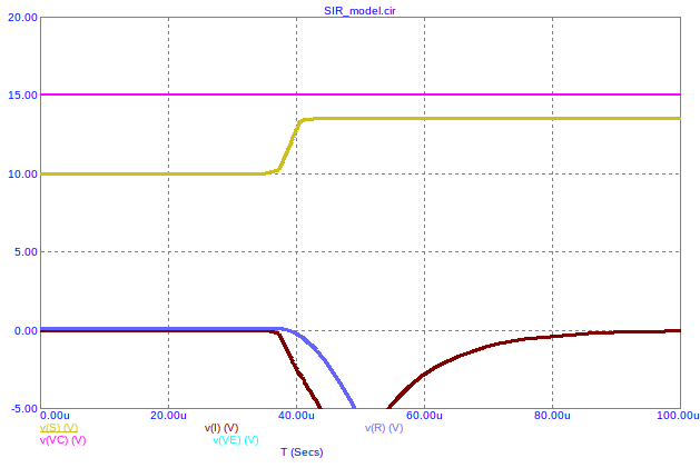
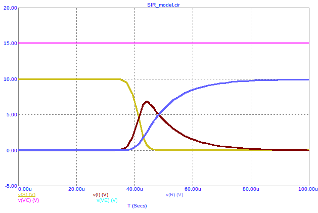
And here is a graph of one run5:
TODO Building a real circuit
When building a real circuit for this model the integrator capacitors will need to be reset to a known voltage at the beginning of each run. In this case, the initial voltages on the capacitors could be zero, and noise might be sufficient for the simulation to start.
The circuit should be reset often in order for the output to rapidly update on an oscilloscope. This way, parameters can be tweaked with potentiometers in real-time to watch the model behavior change.
Footnotes:
My biggest example of going through the motions in college was passing Linear Systems of Differential Equations (MATH309, now called "Linear Analysis"), which combined matrix algebra and differential equations. Every homework problem was essentially the same: find the eigenvalues of a 3x3 matrix by hand, plug them into one of a few formulas, and simplify the result. Each one took about a page of work, but it was straight symbolic manipulation without fundamentally understanding what an eigenvalue was or how the equations represented the system behavior (heat flow in a rod, usually).
To be more precise, the equations are:
\begin{align*} S(t) &= \int_0^t \frac{-\beta}{N} I S dt \\ I(t) &= \int_0^t \frac{\beta}{N} I S - \gamma I dt \\ R(t) &= \int_0^t \gamma I dt \end{align*}Technically, the constants of integration would only appear after replacing the integral expressions with their actual antiderivative functions (assuming they exist in analytical form). But since the constants are arbitrary anyway, there's no harm in including them here. Additionally, we're not attempting to find analytical forms either. This circuit is essentially performing a "numerical" integration.
Also notice that the difference of integrals expression for \(I\) is equivalent to \(I=(N-S)-R\), which confirms our choice of initial conditions since the sum of the sub-populations is indeed \(N\).
Full disclosure: I think I got lucky with the initial conditions here. Changing the \(N\) voltage very slightly (10.01V vs 10V) causes the simulator to settle on a different operating point (initial conditions) which doesn't generate valid graphs. I'll have to learn more about how to better specify initial conditions in the simulator to fix this. Micro-Cap 12 has five different algorithms for determining the initial operating point, but they all exhibit this behavior, which leads me to think my schematic isn't well formed. And perhaps this will be an issue for a physical circuit build as well.